6 Common Probability Inequalities

#MarkovInequality #ChebyshevInequality #CauchySchwarzInequality #ChernoffInequality #HoeffdingInequality #MGF

Problem of the Day:

Pasted image 20241129000220.png|400
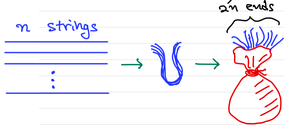
Suppose you tie two free ends u.a.r and continue until no more free ends remain. What is the expected number of loops formed?
Denote $L$ as number of loops formed. Suppose currently there are $K$ open strings. Then we have to tie $K$ times. For the $k$ th time, if a new loop is formed, then denote $I_{k} = 1$ . Else $I_{k} = 0$ . Then $L = I_{n} + I_{n - 1} + \dots + I_{1},$ so $E [L] = \sum_{k = 1}^{n} E [I_{k}] = \sum_{k = 1}^{n} P (I_{k} = 1) .$
Since there are $2 K$ free ends, $P (I_{k} = 1) = \frac{k}{(\binom{2 k}{2})} = \frac{1}{2 k - 1},$ so $E [L] = \sum_{k = 1}^{n} \frac{1}{2 k - 1} \sim \frac{1}{2} \ln n .$

1 Boole's Inequality

By disjoint additivity we can compute $P (A_{1} \cup A_{2}) = P (A_{1}) + P (A_{2}) - P (A_{1} \cup A_{2}) .$
Actually we have the general Inclusion-Exclusion Principle: $\begin{matrix} (1.1) & P (⋃_{i = 1}^{n} A_{i}) = Σ_{1} - Σ_{2} + Σ_{3} - Σ_{4} + \dots + (- 1)^{n - 1} Σ_{n}, \end{matrix}$ where $Σ_{k} = \sum_{1 \leq i_{1} < \dots < i_{k} \leq n} P (A_{i_{1}} \dots A_{i_{k}})$ , which can be proved by induction and definition. However we can have a neater result when it comes to inequality:

Theorem (Union Bound, Boole's Inequality)

$A_{1}, \dots, A_{n} \in F$ are a collection of events on a probability space $(Ω, F, P)$ . Then $P (⋃_{i = 1}^{n} A_{i}) \leq \sum_{i = 1}^{n} P (A_{i}) .$

This can be proved by induction on $n$ and (1.1), so is omitted.

2 Cauchy-Schwarz Inequality

Theorem (Cauchy-Schwarz Inequality)

Let $X, Y$ be two RVs on the same probability space. Then $(E [X Y])^{2} \leq E [X^{2}] E [Y^{2}],$ i.e. $(Cov (X, Y))^{2} \leq Var (X) Var (Y) .$

Proof

For constants $a, b \in R$ , $\begin{aligned} 0 \leq E [(a X - b Y)^{2}] = E [a^{2} X^{2} + b^{2} Y^{2} - 2 a b X Y] \\ \Rightarrow & 2 a b E [X Y] \leq a^{2} E [X^{2}] + b^{2} E [Y^{2}] . \end{aligned}$
Let $a = \sqrt{E [Y^{2}]}, b = \sqrt{E [X^{2}]}$ , then $E [X Y] \leq \sqrt{E [X^{2}] E [Y^{2}]} .$
Similarly, the other side can be proved by $0 \leq E [(a X + b Y)^{2}]$ .

3 Concentration Inequalities

We often want to estimate the tail, i.e. $P (X \geq c)$ or $P (| X - μ | \geq c)$ . This is important for proving convergence results, bounding failure probabilities, or probabilistic bounds on runtimes.

3.1 Markov's Inequality

Theorem (Markov's Inequality)

Let $X$ be a non-negative RV with $E [| X |] < \infty$ . Then for any constant $c > 0$ , $P (X \geq c) \leq \frac{E [X]}{c} .$

Proof

Lemma

X is a non-negative RV, then $\forall ω \in Ω, \forall c > 0$ , $X (ω) \geq c I_{{X \geq c}} (ω)$ .

Recall indicator RV: for $A \in F$ , $I_{A} (ω) = {\begin{aligned} 1, ω \in A, \\ 0, ω \notin A . \end{aligned}$
$(I_{A} = 1) = {ω \in Ω | I_{A} = 1} = A$ , so $E [I_{A}] = P (I_{A} = 1) = P (A)$ .

Proof of Lemma

$(X \geq c) = {ω \in Ω | X (ω) \geq c}$ .

If $X (ω) < c$ , $I_{{X \geq c}} (ω) = 0$ . And $X$ non-negative, so $X (ω) \geq 0, \forall ω \in Ω$ . Then result holds.
If $X (ω) \geq c$ , $I_{{X \geq c}} (ω) = 1$ . Also holds.

By the lemma, $\forall ω \in Ω, c > 0$ , $X (ω) \geq c I_{{X \geq c}} (ω)$ . Take expectation: $E [X] \geq E [c I_{{X \geq c}}] = c P (X \geq c) .$

Theorem (Generalized Markov's Inequality)

Let $X : Ω \to R$ be an arbitrary RV. Then for all constants $c > 0, k > 0$ , $P (| X | \geq c) \leq \frac{E [| X |^{k}]}{c^{k}} .$

Proof

Similar argument as above, applied to $| X (ω) |^{k} \geq c^{k} I_{{| X | \geq c}} (ω)$ .

3.2 Chebyshev's Inequality

Theorem (Chebyshev's Inequality)

For all RVs $X$ with $E [X] = μ < \infty$ and for all constants $c > 0$ , $P (| X - μ | \geq c) \leq \frac{Var (X)}{c^{2}} .$

Proof

Since $| X - μ | \geq c ⟺ | X - μ |^{2} \geq c^{2}$ , $P (| X - μ | \geq c) = P (| X - μ |^{2} \geq c^{2}) \leq \frac{E [| X - μ |^{2}]}{c^{2}} = \frac{Var (X)}{c^{2}} .$
Here we applied Markov's Inequality.

3.3 Chernoff Inequalities

Theorem (Chernoff Inequalities)

A one-parameter family of bounds derived as follows:

$\forall t > 0, c \in R$ , $P (X \geq c) \leq min_{t > 0} \frac{M_{X} (t)}{e^{t c}} .$
$\forall t < 0, c \in R$ , $P (X \leq c) \leq min_{t < 0} \frac{M_{X} (t)}{e^{t c}} .$

Proof

For $t > 0$ case, by Markov's inequality $P (X \geq c) = P (e^{t X} \geq e^{t c}) \leq \frac{E [e^{t X}]}{e^{t c}} = \frac{M_{X} (t)}{e^{t c}} .$
(Check definition of MGF) Since LHS is irrelevant of $t$ , we can take minimal to $t$ . Similar for $t < 0$ .

Example

If $X \sim Binomial (n, p), I \sim Bernoulli (p)$ , then $E [X] = n p$ . $M_{X} (t) = [M_{I} (t)]^{n} = [e^{t} p + (1 - p)]^{n} .$
For $t > 0$ , $P (X \geq a n) \leq \frac{[e^{t} p + (1 - p)]^{n}}{e^{a n t}}$ . Take derivative to find the minimum point $\frac{d}{d t} RHS (t) = \frac{n [e^{t} p + (1 - p)]^{n - 1} (e^{t} p) - a n [e^{t} p + (1 - p)]^{n}}{e^{a n t}} .$
Let it be $0$ , then $e^{t} = \frac{a (1 - p)}{p (1 - a)}$ . Plug in Chernoff Inequalities, we have $P (X \geq a n) \leq {(\frac{1 - p}{1 - a})}^{(1 - a) n} {(\frac{p}{a})}^{a n} .$

For $p = \frac{1}{2}, a = \frac{3}{4}$ , this yields $P (X \geq \frac{3 n}{4}) \leq {(\frac{16}{27})}^{\frac{n}{4}}$ . This is much stronger than:

Markov's inequality: $P (X \geq \frac{3 n}{4}) \leq \frac{2}{3}$ ,

Chebyshev's inequality: $\begin{aligned} P (X \geq \frac{3 n}{4}) & = P (X - \frac{n}{2} \geq \frac{n}{4}) \\ \leq P (| X - \frac{n}{2} | \geq \frac{n}{4}) \leq \frac{4}{n} . \end{aligned}$

3.4 Hoeffding's Inequality

This inequality is specific for bounded RVs.

Theorem (Hoeffding's Inequality)

Let $X_{1}, \dots, X_{n}$ be independent RVs with $E [X_{i}] = μ_{i} < \infty$ , and $P (a_{i} \leq X_{i} \leq b_{i}) = 1$ for some constants $a_{i}, b_{i} \in R$ . Let $S_{n} = X_{1} + \dots + X_{n}$ , then $\forall ε > 0$ , $P (| S_{n} - E [S_{n}] | \geq ε) \leq 2 \exp [\frac{- 2 ε^{2}}{\sum_{i = 1}^{n} (b_{i} - a_{i})^{2}}] .$
Equivalently, $P (| \frac{S_{n}}{n} - \frac{E [S_{n}]}{n} | \geq ε) \leq 2 \exp [\frac{- 2 ε^{2} n^{2}}{\sum_{i = 1}^{n} (b_{i} - a_{i})^{2}}] .$

Hoeffding's bound only depends on the range of $X_{i}$ , not its distribution over $[a_{i}, b_{i}]$ . Using more information about $X_{i}$ can lead to a sharper bound, like Chernoff.

Proof

First, recall MGF for normal distribution. Let $X \sim N (μ, σ^{2})$ , with p.d.f $f_{X} (x) = \frac{1}{\sqrt{2 π σ^{2}}} e^{- \frac{(x - μ)^{2}}{2 σ^{2}}}$ . Then $\forall t \in R$ , $M_{X} (t) = E [e^{t X}] = \int_{- \infty}^{+ \infty} \frac{1}{\sqrt{2 π σ^{2}}} e^{t x} e^{- \frac{(x - μ)^{2}}{2 σ^{2}}} d x = e^{t μ + \frac{t^{2} σ^{2}}{2}} .$

Sub-Gaussian

A RV $X$ with $E [X] = μ < \infty$ is said to be sub-Gaussian with variance proxy $σ^{2} > 0$ , if $E [e^{t (X - μ)}] \leq e^{\frac{t^{2} σ^{2}}{2}}, \forall t \in R .$

Lemma1

Let $X$ be a sub-Gaussian RV with $E [X] = μ < \infty$ and variance proxy $σ^{2}$ . Then $\forall ε > 0$ , $P (| X - E [X] | \geq ε) \leq 2 e^{- \frac{ε^{2}}{2 σ^{2}}} .$

Proof of Lemma 1

By Chernoff inequalities, $\forall t > 0$ , $P (X - μ > ε) \leq \frac{E [e^{t (X - μ)}]}{e^{t ε}} \leq \frac{e^{t^{2} σ^{2} / 2}}{e^{t ε}} \equiv g (t),$ where the second " $\geq$ " is derived from lemma assumption. We know by taking derivative, $g (t)$ is minimized at $t = \frac{ε}{σ^{2}}$ . Plug it in: $P (X - μ > ε) \leq e^{- \frac{ε^{2}}{2 σ^{2}}} .$
Similarly, $\forall t < 0$ , $P (X - μ < - ε) \leq \frac{E [e^{t (X - μ)}]}{e^{- t ε}} \leq \frac{e^{t^{2} σ^{2} / 2}}{e^{- t ε}} .$
So $P (| X - μ | \geq ε) = P (X - μ \geq ε) + P (X - μ \leq - ε) \leq 2 e^{- \frac{ε^{2}}{2 σ^{2}}} .$

Lemma2 (Hoeffding's Lemma)

Let $X$ be a RV s.t. $E [X] = μ < \infty$ and $P (a \leq X \leq b) = 1$ for some constants $a, b \in R, a < b$ . Then $E [e^{t (X - μ)}] \leq e^{\frac{t^{2}}{2} {(\frac{b - a}{2})}^{2}}, \forall t \in R .$ i.e. sub-Gaussian with variance proxy $σ^{2} = {(\frac{b - a}{2})}^{2}$ .

Proof of Lemma 2

Let $Y = X - μ$ and $φ (t) = \log E [e^{t Y}]$ ( $φ (0) = 0$ ). Then $\frac{d φ (t)}{d t} = \frac{E [Y e^{t Y}]}{M_{Y} (t)}, \frac{d^{2} φ (t)}{d t^{2}} = \frac{E [y^{2} e^{t Y}]}{M_{Y} (t)} - {(\frac{d φ}{d t})}^{2} .$ ( ${\frac{d φ (t)}{d t} |}_{t = 0} = E [X - μ] = 0$ )
Define a probability measure $P_{t} (y \leq Y \leq y + d y) = \frac{e^{t y}}{M_{Y} (t)} P (y \leq Y \leq y + d y) .$ ( $P_{0} = P$ ). Then $\begin{aligned} \frac{d φ (t)}{d t} & = E_{t} [Y], \\ \frac{d^{2} φ (t)}{d t^{2}} & = E_{t} [Y^{2}] - (E_{t} [Y])^{2} = {Var}_{t} (Y) = {Var}_{t} (Y - \frac{a + b}{2} + μ) \\ \leq E_{t} [{(X - \frac{a + b}{2})}^{2}] \leq {(\frac{b - a}{2})}^{2}, \end{aligned}$ the last " $\leq$ " holds because $\begin{aligned} 1 & = P (a \leq X \leq b) = P (- \frac{b - a}{2} \leq X - \frac{a + b}{2} \leq \frac{b - a}{2}) \\ = P (| X - \frac{a + b}{2} | \leq \frac{b - a}{2}) . \end{aligned}$ Then $φ (t) \leq \frac{t^{2}}{2} {(\frac{b - a}{2})}^{2}$ . Since $\exp$ is monotonically increasing, $E [e^{t Y}] \leq e^{\frac{t^{2}}{2} {(\frac{b - a}{2})}^{2}}$ .

Given the above two lemmas, we can prove Hoeffding's inequality.
First, since $\begin{aligned} E [\exp^{t (S_{n} - \sum_{i = 1}^{n} μ_{i})}] & = E [\prod_{i = 1}^{n} e^{t (X_{i} - μ_{i})}] = \prod_{i = 1}^{n} E [e^{t (X_{i} - μ_{i})}] \\ \leq \prod_{i = 1}^{n} e^{\frac{t^{2}}{2} {(\frac{b_{i} - a_{i}}{2})}^{2}} = e^{\frac{t^{2}}{2} \sum_{i = 1}^{n} {(\frac{b_{i} - a_{i}}{2})}^{2}}, \end{aligned}$
(" $\leq$ " by lemma 2) so $S_{n}$ is sub-Gaussian with variance proxy $σ^{2} = \sum_{i = 1}^{n} \frac{(b_{i} - a_{i})^{2}}{4}$ .
Next, let $X = S_{n}$ and apply lemma 1, we complete the proof.